X-ray Absorption Spectroscopy L-edge Spectrum Simulation
In this tutorial we will simulate the X-ray Absorption Spectroscopy (XAS) L-edge spectrum of the [FeCl4]2− ion using the protocol developed by Chantzis et al.1 This protocol consists of two main parts:
1- Valence orbitals optimization;
2- CASCI calculation with excitations from the Fe 2*p* orbitals to the optimized valence orbitals.
Valence orbital optimization
In this first step, we will perform a CASSCF calculation aiming to prepare the orbitals to receive the core electrons (Fe 2*p*). The ground state configuration for this system is e3 t23 (S = 2). In this regard, the minimum active space would include those six electrons in the five Fe 3*d* orbitals. However, it is known that the inclusion of ligand orbitals into the active space improves the excitation energies, and consequently, the final spectrum.2 Therefore, we will perform a SA-CASSCF(8,7) including 6 roots for S = 2, and 43 roots for S = 1:
```bash title="FeCl4_2-_fci_orbprep.inp" linenums="1"
General
  CalcType CASSCF
  Ints RI
  Basis def2-SVP
  AuxBasis def2-JK
  Charge -2
  Mult 5 3
  OrbGuessName inporbs.C0
End

CASSCF
  NEl 8
  NOrb 7
  NRoots 6 43
  CISolver FCI
  OrbStep FNR
  MaxIter 150
  NRMaxIter 150
  PTCanonStep SA
End

Plot
  Orbs 44 45 46 47 48 49 50
  GridPoints 90 90 90
End

Geom
  Fe         -0.00000189748474     -0.00017731428014     -0.00000000775753
  Cl         -0.00000148327523     -2.03063462815079      1.24686979132265
  Cl          2.03035858590062     -0.00008402467458     -1.24702478912376
  Cl         -0.00000195841589      2.03008677053448      1.24717930723389
  Cl         -2.03036273356026     -0.00008354966590     -1.24702442033183
End
```
How many roots should I calculate?
In this protocol, the authors recommend optimizing the active space to include valence excited
states within the range of 6 to 15 eV. As a general guideline for optimizing XAS L-edge spectra, it is advised to examine the full width at half maximum (FWHM) of the experimental L3 band. Consequently, sufficient roots should be calculated for each spin multiplicity to match the experimental FWHM.
For this calculation, the valence excited states range from 0 to 12 eV, and 0 to 5 eV for S = 2 and S = 1, respectively.
CASSCF State and Excitation Energies Output Example
Following is a sample output:
  ```bash title="FeCl4_2-_fci_orbprep.out"
     CASSCF state and excitation energies:
     Multiplicity 5
        Root    E (var) [Ha]        dE (0->n) [eV]      Oscillator str.
        0       -3099.94231009
        1       -3099.93270828      0.261278            0.000000
        2       -3099.92580344      0.449169            0.000011
        3       -3099.92569550      0.452106            0.000008
        4       -3099.92006356      0.605359            0.000085
        5       -3099.51923277      11.512519           0.000009
     Multiplicity 3
        Root    E (var) [Ha]        dE (0->n) [eV]      Oscillator str.
        0       -3099.84828527
        1       -3099.84437931      0.106287            0.000000
        2       -3099.84428309      0.108905            0.000000
        3       -3099.84044818      0.213258            0.000000
        4       -3099.83633922      0.325069            0.000009
        5       -3099.83401351      0.388354            0.000001
        6       -3099.83385969      0.392540            0.000001
        7       -3099.83315728      0.411654            0.000000
        8       -3099.83079080      0.476049            0.000000
        9       -3099.83028588      0.489788            0.000001
        10      -3099.83008376      0.495288            0.000001
        11      -3099.82295116      0.689376            0.000001
        12      -3099.82277983      0.694038            0.000001
        13      -3099.82250957      0.701393            0.000021
        14      -3099.82149114      0.729105            0.000000
        15      -3099.81774957      0.830919            0.000003
        16      -3099.81772991      0.831454            0.000003
        17      -3099.81486023      0.909542            0.000000
        18      -3099.81418040      0.928041            0.000000
        19      -3099.80909196      1.066504            0.000000
        20      -3099.80879607      1.074556            0.000027
        21      -3099.80865972      1.078266            0.000028
        22      -3099.80786602      1.099864            0.000046
        23      -3099.80712878      1.119925            0.000002
        24      -3099.80588292      1.153827            0.000000
        25      -3099.80588123      1.153873            0.000000
        26      -3099.80453130      1.190606            0.000000
        27      -3099.79904010      1.340029            0.000008
        28      -3099.79880472      1.346434            0.000008
        29      -3099.79762748      1.378469            0.000000
        30      -3099.77464884      2.003749            0.000104
        31      -3099.77214982      2.071751            0.000000
        32      -3099.76936206      2.147610            0.000019
        33      -3099.76914729      2.153454            0.000020
        34      -3099.76773225      2.191959            0.000000
        35      -3099.67842610      4.622103            0.000147
        36      -3099.67798999      4.633970            0.000153
        37      -3099.67443582      4.730684            0.000000
        38      -3099.66789563      4.908652            0.000000
        39      -3099.66725841      4.925991            0.000000
        40      -3099.66638062      4.949877            0.000018
        41      -3099.66572346      4.967760            0.000000
        42      -3099.66223107      5.062792            0.000008
  ```
Starting orbitals for the valence orbital optimization
The concept of valence orbital optimization involves selecting an active space composed of
singly-occupied and unoccupied orbitals that will accommodate the core electrons, along with a few significant ligand orbitals. Consequently, AVAS orbitals featuring the d-valence orbitals or ASS1ST orbitals are appropriate as starting orbitals for this calculation.
CASCI calculation
The figure below shows the active space obtained in the previous step:
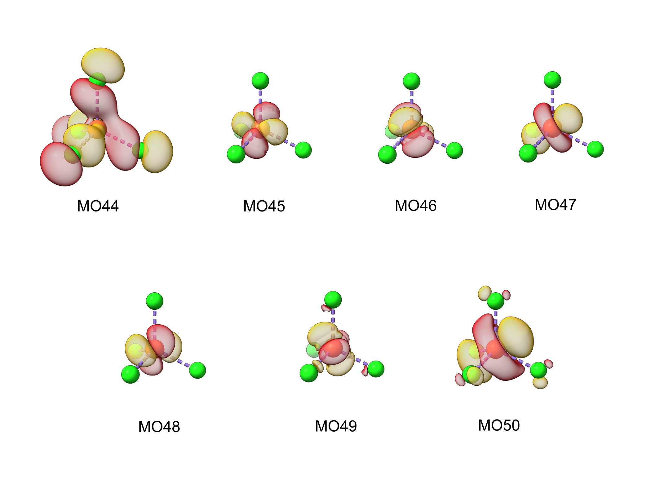
To perform the CASCI calculation, firstly we have to rotate the Fe 2*p* orbitals into the active space. Therefore, we have to rotate the MOs 6, 7, and 8 into the active space.
Fe 2*p* orbitals
Following is a sample output:
  ```bash title="FeCl4_2-_fci_orbprep.out"
                                                      ---------------------
                                                      | INTERNAL ORBITALS |
                                                      ---------------------

  ------------------------------------------------------------------------------------------------------------------------
        0                       1                       2                       3                       4
   -260.1364               -104.3920               -104.3913               -104.3844               -103.7394
     2.0000                  2.0000                  2.0000                  2.0000                  2.0000
  ------------------------------------------------------------------------------------------------------------------------
  1.00      s/Fe0         0.25      s/Cl3         0.25      s/Cl3         0.28      s/Cl2         0.28      s/Cl1
  0.00      s/Cl2         0.25      s/Cl4         0.25      s/Cl4         0.28      s/Cl4         0.28      s/Cl3
  0.00      s/Cl4         0.25      s/Cl2         0.25      s/Cl1         0.22      s/Cl1         0.22      s/Cl2
  0.25      s/Cl1         0.25      s/Cl2         0.22      s/Cl3         0.22      s/Cl4
  ------------------------------------------------------------------------------------------------------------------------

  ------------------------------------------------------------------------------------------------------------------------
        5                       6                       7                       8                       9
    -31.2507                -27.0953                -27.1050                -27.0775                -10.1522
     2.0000                  2.0000                  2.0000                  2.0000                  2.0000
  ------------------------------------------------------------------------------------------------------------------------
  0.98      s/Fe0         0.56     px/Fe0         0.56     py/Fe0         1.00     pz/Fe0         0.25      s/Cl2
  0.00     py/Cl4         0.44     py/Fe0         0.44     px/Fe0         0.00     py/Cl1         0.25      s/Cl3
  0.00     px/Cl3         0.00      s/Fe0         0.00      s/Fe0         0.00     px/Cl2         0.25      s/Cl1
  0.25      s/Cl4
  ------------------------------------------------------------------------------------------------------------------------
  ...
  ```
The input for this calculation is:
```bash title="FeCl4_2-_casci14e10o.inp" linenums="1" hl_lines="8-11 16-17 21"
General
  CalcType CASSCF
  Ints RI
  Basis def2-SVP
  AuxBasis def2-JK
  Charge -2
  Mult 5 3
  OrbGuessName inporbs_cas8e7o.C0
  OrbGuessRotation 6 41 90
  OrbGuessRotation 7 42 90
  OrbGuessRotation 8 43 90
  Temperature 300
End

CASSCF
  NEl 14
  NOrb 10
  NRoots 170 650
  CISolver FCI
  OrbStep FNR
  MaxIter 0
  NRMaxIter 150
  PTCanonStep SA
  DoSOC true
End

Geom
  Fe         -0.00000189748474     -0.00017731428014     -0.00000000775753
  Cl         -0.00000148327523     -2.03063462815079      1.24686979132265
  Cl          2.03035858590062     -0.00008402467458     -1.24702478912376
  Cl         -0.00000195841589      2.03008677053448      1.24717930723389
  Cl         -2.03036273356026     -0.00008354966590     -1.24702442033183
End
```
Some important notes about the input file:
* The guess orbitals for this calculation come from the valence orbital optimization step;
* The Fe 2*p* orbitals are exchanged with the MOs immediately before the active space, i.e. MOs
41, 42, and 43. Consequently, the active space for this calculation consists of 14 electrons
(6xFe 2*p* + 8) and 10 orbitals (3xFe 2*p* + 7);
* To perform a CASCI calculation, the MaxIter keyword must be set as 0.
Important Note
Due to the number of roots necessary to do this calculation, it is advisable to run this
calculation in a computer cluster.
Tip: make sure that the Fe 2*p* orbitals are in the active space
To make sure that the Fe 2*p* orbitals are in the active space, the following lines can be added to the input file:
```bash title="FeCl4_2-_casci14e10o.inp"
Plot
  Orbs 41 42 43 44 45 46 47 48 49 50
  GridPoints 90 90 90
End
```
The final spectrum for this calculation is shown bellow:
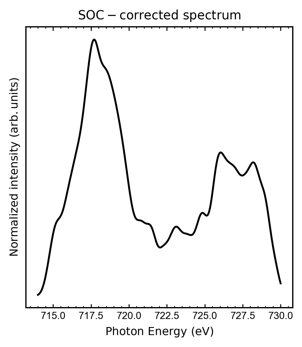
The bands for this spectrum were convoluted using Gaussian functions with FWHM = 0.7 eV. As one can see, the two main features of a XAS L-edge spectrum are reproduced: the L3 and L2 bands. Further improvements can be reached by including NEVPT2 calculations on top of the CASCI calculation.
Shifts to reach better match with experimental spectrum
Due to the approximations employed in quantum chemical calculations, generally the excitation
energies should be shifted to achieve a better match with the experimental spectrum. In this case, a shift of -11 eV would provide a better match with the experimental spectrum.
Here you can download the inputs, outputs, and starting orbitals used in this tutorial:
- Valence orbital optimization:
- CASCI calculation: